Propensity score matching in Python, revisited

Update 8/11/2017: I’ve been working on turning this code into a package people can download and contribute to. Please use the package, linked here, instead of the code I shared in a Jupyter notebook previously.

I can’t believe how many people from all around the world visit my previous blog post on propensity score matching in Python every day.  It feels great to know that my code is out there and people are actually using it.  However, I realized that the notebook I link to previously doesn’t contain much and that I wrote heaps more code after posting it.  Hence, I’m sharing a more complete notebook with code for different variations on propensity score matching, functions to compute average treatment effects and get standard errors, and check for balance between matched groups.

Estimation vs. Inference

I went to Marti Anderson’s talk at UC BIDS yesterday where she introduced a generalization of mixed model ANOVA which uses a correction factor in the estimation which essentially corrects for how random your random effects are.  She showed that if your random effects are actually close to fixed, then you gain statistical power by setting the correction factor close to 0.  This was all good until after the talk, somebody asked a question to the effect of “well I thought the big difference between fixed and random effect models was that your data don’t have to be normal for fixed effects, so how does that come into play here?”

The answer: it doesn’t.  Nowhere in her talk did Marti mention a normality assumption the data.  P-values for the were computed using permutation tests, which make no assumptions about the underlying distribution of your data.  All you need to use a permutation test is an invariance or symmetry assumption about your data under the null hypothesis: for example, if biological sex had no relation to height, then the distributions of male and female heights should be identical and we relabeled people male or female at random, the height distributions wouldn’t change.

People often confuse the assumptions needed to estimate parameters from their models and the assumptions to create confidence intervals and do hypothesis tests.  The most salient example is linear regression.  Even without making any assumptions, you can always fit a line to your data.  That’s because ordinary least squares is just an estimation procedure: given covariates X and outcomes Y, all you need to do is solve a linear equation.  Does that mean your estimate is good?  Not necessarily, and you need some assumptions to ensure that it is.  These are that your measurement errors are on average 0, they have the same variance (homoskedasticity), and they’re uncorrelated.  Then your regression line will be unbiased and your coefficient estimates will be “best” in a statistical sense (this is the Gauss-Markov theorem).  Of course, for this to work you also need more data points than parameters, no (near) duplicated covariates, and a linear relationship between Y and X, but hopefully you aren’t trying to use ordinary least squares if these don’t hold for your data!

Notice that there are no normality assumptions for the Gauss-Markov theorem to hold; you just need to assume a few things about the distribution of your Y data that can sort of be checked.  Normal theory only comes into play if you want to use “nice” well-known distributions to construct confidence intervals.  If you assume your errors are independent and identically distributed Gaussian mean-0 noise with common variance, then you can carry out F-tests for model selection and use the t-distribution to construct confidence intervals and to test whether your coefficients are significantly different from 0.

This is what usual statistical packages spit out at you when you run a linear regression, whether or not the normality assumptions hold.  The estimates of the parameters might be ok regardless, but your confidence intervals and p-values might be too small.  This is where permutation tests come in: you can still test your coefficients using a distribution-free test.

As an example, I’ve simulated data and done ordinary least squares in R, then compared the output of the lm function to the confidence intervals I construct by permutation tests.*  I’m just doing a simple univariate case so it’s easy to visualize.  The permutation test will test the null hypothesis that the regression coefficient is 0 by assuming there is no relationship between X and Y, so pairs are as if at random.  I scramble the order of the Xs to eliminate any relationship between X and Y, then rerun the linear model.  Doing this 1000 times gives an approximate distribution of regression coefficients if there were no association.

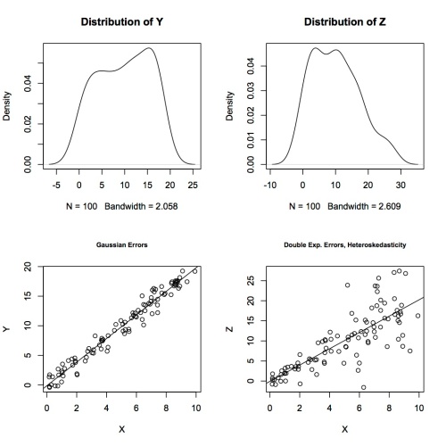
I generated 100 random X values, then simulated errors in two ways.  First, I generated independent and identically distributed Gaussian errors e1 and let Y=2X + e1. I ran linear models and permutation tests for both to get the following 95% confidence intervals:

> confint(mod1,2) # t test
2.5 % 97.5 %
X 1.917913 2.068841
> print(conf_perm1) # permutation test
X X
1.598273 2.388481


When the normality assumptions are true, then we get smaller confidence intervals using the t-distribution than using permutation tests. That makes sense – we lose efficiency when we ignore information we know.

Then I generated random double exponential (heavy-tailed distribution) errors e2 that increase with X, so they break two assumptions for using t-tests for inference, and let Z = 2X + e2.  The least squares fit is very good, judging by the scatterplot of Z against X – the line goes right through the middle of the data.  There’s nothing wrong with the estimate of the coefficient, but the inference based on normal theory can’t be right.

> confint(mod2,2) # t test
2.5 % 97.5 %
X 1.716465 2.348086
> print(conf_perm2) # permutation test
X X
1.531020 2.533531


Again, we get smaller confidence intervals for the t-test, but these are simply wrong.  They are artificially small because we made unfounded assumptions in using the t-test intervals; perhaps this points to one reason why so many research findings are false.  It’s this very reason that it’s important to keep in mind what assumptions you’re making when you carry out statistical inference on  estimates you obtain from your data – nonparametric tests may be the way to go.

* My simulation code is on Github.

Tips for efficiency at the command line

The terminal can be a powerful tool in statistical computing.  I’ve used UNIX a bit before, mostly just to run jobs on remote servers and handle giant files.  I know how to copy files, move them between folders, edit text files in Emacs, and use simple commands like grep and cut along with pipes and filters to sift through files.  I wouldn’t say I’m savvy by any means, but I know enough to get by.  I’m always looking for tips to maximize my speed while minimizing the work I have to do.  This week I learned a few things that I thought were useful for getting more out of the terminal as a tool for research.  In particular, some of the things I learned facilitate reproducibility, which is becoming increasingly important and rare.

– Aliasing: There are probably things you type repeatedly at the command line, like your username when logging into remote machines or cd to a certain frequently used directory. You can save time typing these things over and over again by creating an “alias” for them in the terminal. This essentially means you create a shortcut to call this command, instead of writing out the whole thing. For instance, I might write something like

alias jobs="top -u kellie"

Then, when I type jobs, I will see the CPU, % Memory, and run time for any jobs I have running and ignore the processes that belong to other users.  It’s a clever trick that might save me 1 second each time I use it.

Now, that’s nice to have in one session, but what if you want to keep using the same shortcuts every time you open the terminal?  If you just created an alias once and closed the terminal, then it would get discarded.  Every time you open the terminal, the bash shell scans through a file called .bashrc and imports all the variables, aliases and functions within the file.  You can save shortcuts you create by opening the .bashrc file in any text editor and pasting them in.

Note: I use OS X Mavericks and by default, there is no .bashrc file.   I have had luck doing the same thing with the .bash_profile file instead.  To see if you have a .bashrc file in your home directory, run

cd
ls -a | grep ^.bash

– Saving shell code: This one’s probably a no-brainer for some of you, but I didn’t know you could do it!  You can write your shell scripts in a text file and save it with the extension .sh.  You should include #!/bin/bash in the first line of this file. Then, you can run it at the command line by calling ./myfile.sh, where you replace “myfile” with whatever your file is called.

– Command history: Related to the previous point.  You can always press the up arrow to bring to the prompt lines you’ve recently run.  What if you ran a command much earlier in the day and want to do it again, but don’t remember the exact syntax?  Your working directory has a file with your command history in it.  By default, mine contains the last 500 lines I’ve run. You can access it by typing either history to print it all to the screen or less ~/.bash_history to view page by page.

– Variables in the command line:  While there might be more clever ways to pass arguments to functions (like xargs), it’s easy and intuitive do it if you store your argument as a variable.  You can store output of a command by enclosing it in back ticks.  Suppose I have a bunch of csv files of the same format and I want to put the first column of each file into one master file. I would first get the names of all the files I want and store them in a variable called files

files=`ls | grep .csv`

Then you can do something like loop over the files and use >> to append them to the master file.  Compared to something like a string of pipes, this syntax feels intuitive to me because it mimics scripting languages I’m more familiar with.

for file in $files
do
    cut -d',' -f1 $file >> masterfile.csv
done

And of course, you can completely automate this by putting it in a .sh file and running it from the command line!  This is really powerful for facilitating reproducibility.  Often, we download files from the web or do easy text processing and file cleanup like this by hand, but then nobody else can retrace our steps.  Sometimes I can’t even reproduce what I did myself.  This is a clean way to keep track of what has been done (not to mention much faster, once you get things running).